

Introduction
Materials and Methods
Experimental Setup and Measurements
Simulation
Simulation Conditions and Parameters
Statistical Analysis
Results and Discussion
Conclusions
Introduction
Surface drip irrigation is one of the most efficient methods for irrigating vegetables. Because it releases small amounts of water at a high frequency, the water use efficiency is higher. Many researchers have reported high yields and quality of vegetable crops using surface drip irrigation—potato (Wang et al., 2006), eggplant (Colak et al., 2018), cucumber (Yuan et al., 2006), and bell pepper (Sezen et al., 2006). Surface drip irrigation uses emitters and lateral lines laid on the soil surface. An emitter discharges small amounts of water at a controlled rate, and water infiltration occurs in the soil region directly around the emitter. Thus, the soil water content in the plant root zone remains essentially constant. Emitters with close spacing (0.1 ‑ 0.6 m) are frequently used for irrigation of small fruits and vegetables.
Because many farmers use surface drip irrigation, increasing water use efficiency in irrigation is crucial. Realizing the full potential of drip irrigation technology requires optimization of operational parameters, which are the rate of discharge from the emitter, emitter spacing, duration of water application, and placement of drip tubing (Skaggs et al., 2004). In addition, the soil water distribution patterns formed under the emitter are important for designing an optimal drip irrigation system. Numerical simulations of water transport in unsaturated soils have been used extensively owing to the complexity of the coupling of water and heat transport in soils and the difficulties associated with field measurements, especially near the soil surface. HYDRUS-2D can simulate three-dimensional water flow, solute transport, and root water uptake based on finite-element methods of the flow equations (Šimůnek et al., 2012). This program is effective for analyzing design features and managing drip irrigation (Cote et al., 2003; Schmitz et al., 2002). However, the simulation must be compared with experimental results to establish its reliability and to evaluate the physical assumptions involved.
Many experiments and simulations have been conducted on water flow in soil to evaluate the efficiency irrigation systems. Arraes et al. (2019) developed a numerical model that simulates the water distribution and the shape of the wetted soil. However, this research only used a point source as the soil surface dripper. Zhang et al. (2012) measured differences in wetting patterns between a point source and a line source. Some studies using software or experiments have included soil wetting patterns formed during surface drip irrigation (Kandelous and Šimůnek, 2010; Kandelous et al., 2011; Samadianfard et al., 2012; Dabach et al., 2013; Autovino et al., 2018). Although surface drip irrigation has been studied extensively, to our knowledge, no analysis of wetting patterns when using different emitter spacings for horticultural crops has been conducted. Therefore, this study simulates the wetting patterns in surface drip irrigation using the numerical HYDRUS-2D model, compares the values with the experimental data, and assesses the use of simulation in a design drip management system for horticultural crops. This study was carried out using three lateral line spacings (i.e., 20, 40, and 60 cm).
Materials and Methods
Experimental Setup and Measurements
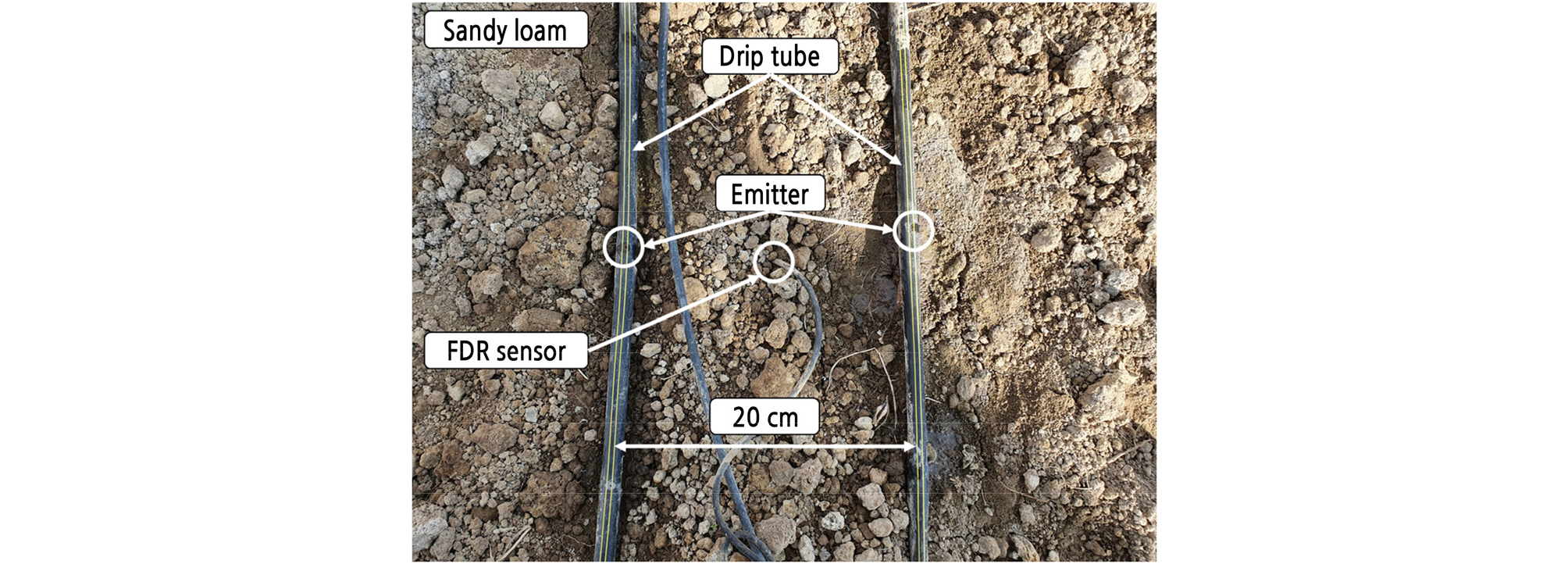
The experimental site (35°29’N, 128°44’E, 14-m altitude) is located at the Department of Southern Area Crop Science, National Institute of Crop Science, Republic of Korea. Each experimental plot, 2 × 2 m square, was originally used as a lysimeter. Table 1 shows the physicochemical properties of the soil studied. The soil texture in this experiment was sandy loam (sand 61.5%, silt 30.5%) (Kim et al., 2018), which quickly drains excess water. Most vegetables grow well in sandy loam soil.
Table 1.
Physico-chemical properties of soil
The wetting patterns of two neighboring emitters eventually overlap to some extent, depending on the emitter spacing. These patterns are also affected by the initial water content and soil properties. However, because the emitter spacing was fixed at 20 cm, the dripline spacing was varied to evaluate the movement of irrigated water between the emitters. As a result, the spacings between two lateral driplines were 20, 40, and 60 cm, which are the common distances for drip irrigation of fruits and vegetables. The emitter discharge rate and the soil texture were 2.1 L/h and sandy loam, respectively.
Soil water content was measured using a frequency domain reflectometry (FDR) sensor (EnviroPro, Entelechy, Australia). This sensor monitors the changes in the dielectric properties of the soil to provide soil moisture. The sensor was installed in accordance with the manufacturer's installation manual to increase the accuracy of the measured values. Any disturbance of soil adjacent to the probe will affect the measurement accuracy. Thus, we confirmed that there were no air gaps or preferential water flow along the probe during the experiment. These 40-cm-long soil probes were installed in the middle of the emitters at adjacent driplines (Fig. 1). The sensors in the soil probe were located at 10-cm increments vertically from the soil surface, i.e., at depths of 10, 20, 30, and 40 cm. This probe was also connected to a data logger, which was programmed to save the data every 10 min. The measured value was adjusted to the value that corresponded to sandy loam soil according to the calibration equation provided by the manufacturer. The measurement accuracy of soil moisture was ± 2%, according to the manufacturer’s manual. In addition, the probes were calibrated for the experimental site by the manufacturer.
In this experiment, a single multi-sensor was used to measure the distribution of soil water. In general, in order to measure water content profiles in the field, several TDR probes were installed vertically or horizontally (Ferre and Topp, 2002; Ramos et al., 2012). By contrast, our FDR probe provided the water content profile from a single installation. Since our study was focused on water infiltration, one sensor for each condition was enough to compare the simulation data; once the discrete measuring data were close to the simulation values, the real water distribution would be similar to the simulation distribution.
This experiment was carried out from 11:00 a.m. on November 6, 2019 to 9:00 a.m. on November 7, 2019 (22 h). Weather data were collected from an automated weather station in the experimental field, and the average temperature and relative humidity were 11°C and 77.1%, respectively. All experiments in this study were performed in triplicate.
Simulation
HYDRUS-2D Model
HYDRUS-2D software (Šimůnek et al., 2012) was used to simulate the two-dimensional movement of water in the soil. Water flow was described using the Richards equation (Richards, 1931).
| $$\frac{\partial\theta(h)}{\partial t}=\frac\partial{\partial x}\left[K(h)\frac{\partial h}{\partial x}\right]+\frac\partial{\partial z}\left[K(h)\frac{\partial h}{\partial z}+K(h)\right]-S(h),$$ | (1) |
where θ is the volumetric water content (cm3 cm-3) in the soil; h is the pressure head (cm); K is the hydraulic conductivity (cm min-1); x and z are the horizontal and vertical coordinates (cm), respectively; t is time (min); and S is the sink term (min-1).
This partial-differential equation governs variably saturated flow in the unsaturated zone. The soil water retention curve and the unsaturated hydraulic conductivity function K(h) were calculated using the van Genuchten ‑ Mualem constitutive relationships (Van Genuchten, 1980).
| $$\theta(h)=\frac{\theta_s-\theta_r}{\lbrack1+\vert\alpha h\vert^n\rbrack^m},$$ | (2) |
| $$K(h)=K_sSe^l\left[1-(1-Se^{l/m})^m\right]^2,$$ | (3) |
where and are the saturated and residual water contents (cm3 cm-3), respectively; (cm-1), n ( ‑ ), and m (=1 ‑ 1/n) (‑) are empirical parameters; Ks is the saturated hydraulic conductivity (cm min-1); and l is the pore connectivity parameter. Se, the degree of saturation, is expressed by the following equation:
| $$S_e=\frac{\theta-\theta_r}{\theta_s-\theta_r}$$ | (4) |
The Richards equation is a nonlinear partial-differential equation. The coefficient of K(h) is a function of the dependent variable . Because of its strong nonlinearity, most practical applications of the Richards equation require a numerical solution.
Simulation Conditions and Parameters
Because the drip tubing had the same emitter spacing (20 cm) and the water was only supplied from the emitters, the emitter was considered a point source. In general, the emitter flux is much greater than the saturated hydraulic conductivity, so the infiltration zone becomes saturated quickly. Therefore, the water flow is symmetrical about the vertical centerline of the emitter. Hence, the soil water distribution patterns at different lateral (drip tubing) spacings would be the same as those at different emitter spacings.
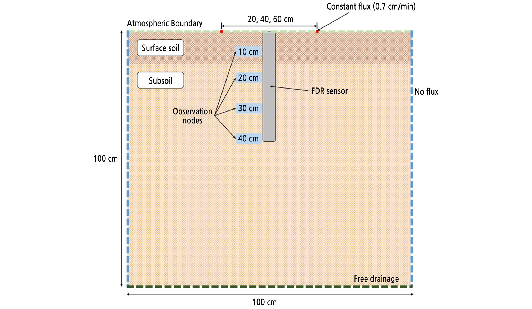
Fig. 2 shows the dimensions in the simulations: the domain was 100 cm wide and 100 cm deep. The Richards equation can be solved numerically with specific initial and boundary conditions. The initial conditions characterize the initial state of the system and are specified in terms of the water content in the vertical direction.
| $$\theta(z,t)=\theta_i(z,0)$$ | (5) |
where (cm3 cm-3) is the initial value of the water content. These initial conditions were uniform in the horizontal direction. The initial conditions were based on the measured data.
At the soil surface, one must account for interactions between the applied water rate and evaporation.
| $$q_o=Q-E_a\mathrm{at}\;\mathrm t>0,\;\mathrm z=0,\;\mathrm x>0,$$ | (6) |
where is the initial flux (cm min-1), Q is the emitter flow rate (cm min-1), and Ea is the actual evaporation rate (cm min-1).
At both lateral boundaries, there was a no-flow condition to account for flow and transport symmetry.
| $$J_w=-K_s\frac{\partial H}{\partial x}=0\;\mathrm{for}\;\mathrm t>0,\;\mathrm z>0$$ | (7) |
Here, Jw is the water flux (cm min-1), Ks is the hydraulic conductivity (cm min-1), and H is the total head (cm).
At the bottom of the soil profile, there is a free drainage condition.
| $$\frac{\partial h}{\partial z}+1=g_o(z,\;t),$$ | (8) |
where go is the prescribed total gradient (cm cm-1). This boundary condition is commonly used when the water table is situated far below the domain of interest.
The soil hydraulic parameters (Table 2) were estimated using the ROSETTA pedotransfer function of Schaap et al. (2001), as implemented in the HYDRUS code. Soil hydraulic properties vary among soils with a textural class. This is especially true near the soil surface, which is affected more by land use and weather (Radcliffe and Šimůnek, 2010). Thus, the soil region was also divided into the surface soil (0 ‑ 15-cm depth) and the subsoil (15 ‑ 100-cm depth). The hydraulic conductivity at the soil surface was higher than that at the subsoil because of the larger porosity in the soil surface region. The emitters were located on the surface, and their discharge rate was 2.1 L/h. Observation nodes were set to a 40-cm depth by increments of 10 cm from the surface (10, 20, 30, and 40 cm). Because the FDR probe was installed in the middle of the emitters, the observing dimension of each node group was set to 6 cm (horizontal direction) by 5 cm (vertical direction) to cover a dielectric-affected area from the FDR sensor. Simulations were performed with three dripline spacings (20, 40, and 60 cm) to investigate the soil water distribution for different drip tube spacings. The soil type was sandy loam in the simulations. The irrigation time in the simulation was 22 h, which is the same as the field experiment, to compare the simulated values with the measured ones.
Table 2.
Properties of soils considered in HYDRUS-2D simulations
| Soil type | (cm-1) | Ks (cm/min) | l | |||
| Surface soil | 0.13 | 0.5 | 0.38 | 2.2 | 0.15 | 0.5 |
| Subsoil | 0.23 | 0.5 | 0.37 | 2.16 | 0.136 | 0.5 |
Statistical Analysis
Statistical tests were employed on the measured and simulated data generated from the field experiment and modeling. The model’s performance was evaluated by comparing measured (M) and HYDRUS-2D simulated (S) values of soil water content. The error between these values was estimated using the root mean square error (RMSE), given by
| $$R\;MSE=\sqrt{\frac1N{\textstyle\sum_{i=1}^N}(M_i-S_i)^2}$$ | (9) |
The coefficient of determination (R2) was also applied to test the proportion of variance in the measured data explained by the model. In addition, the coefficient of efficiency (E) was used to evaluate the performance of the simulation model. The coefficient of efficiency was defined as one minus the ratio of the mean square error to the variance in the observed data (Nash and Sutcliffe, 1970).
| $$E=1-\frac{\sum_{n=1}^N(M_i-S_i)^2}{\sum_{n=1}^N(M_i-\overline M)^2}$$ | (10) |
Results and Discussion
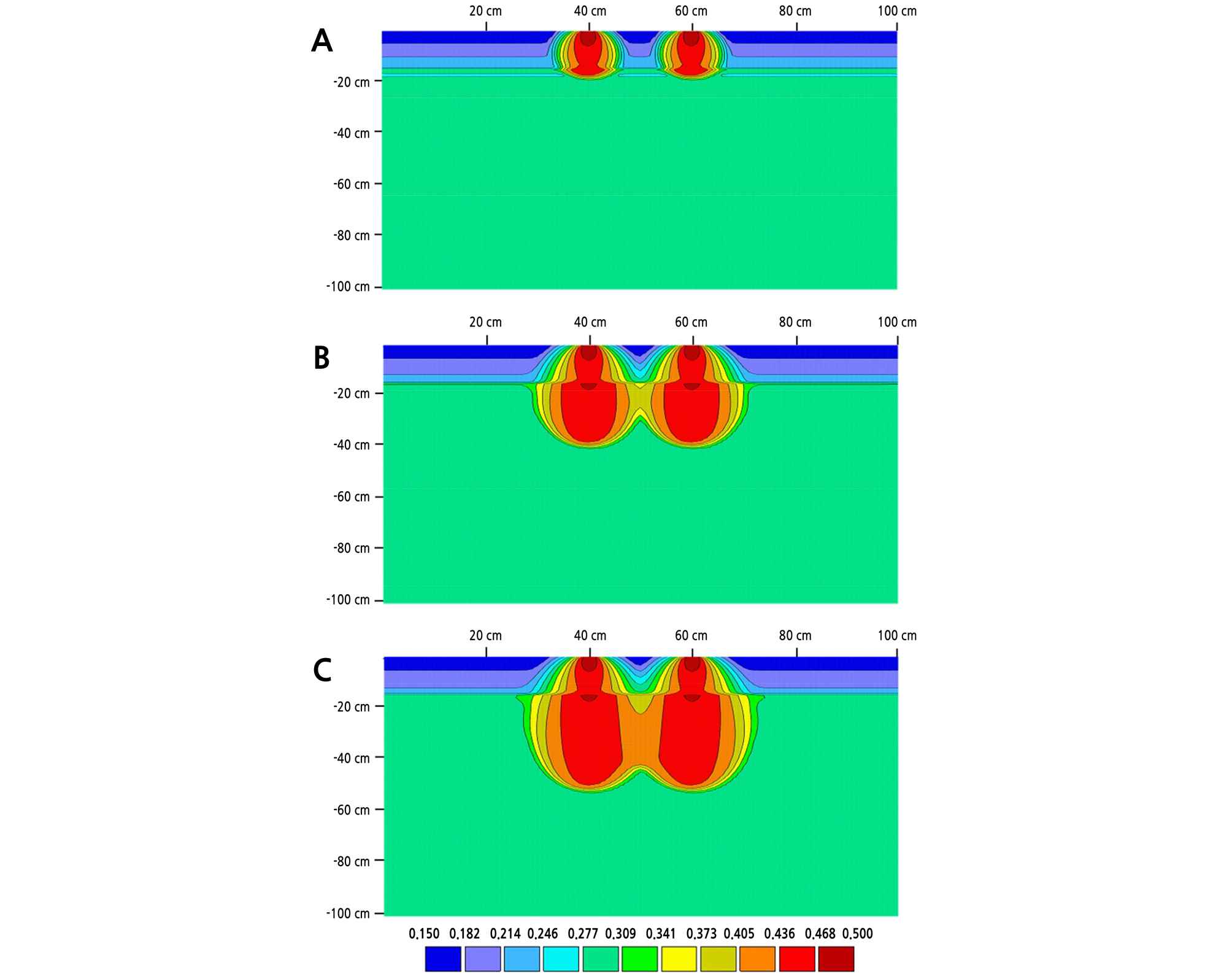
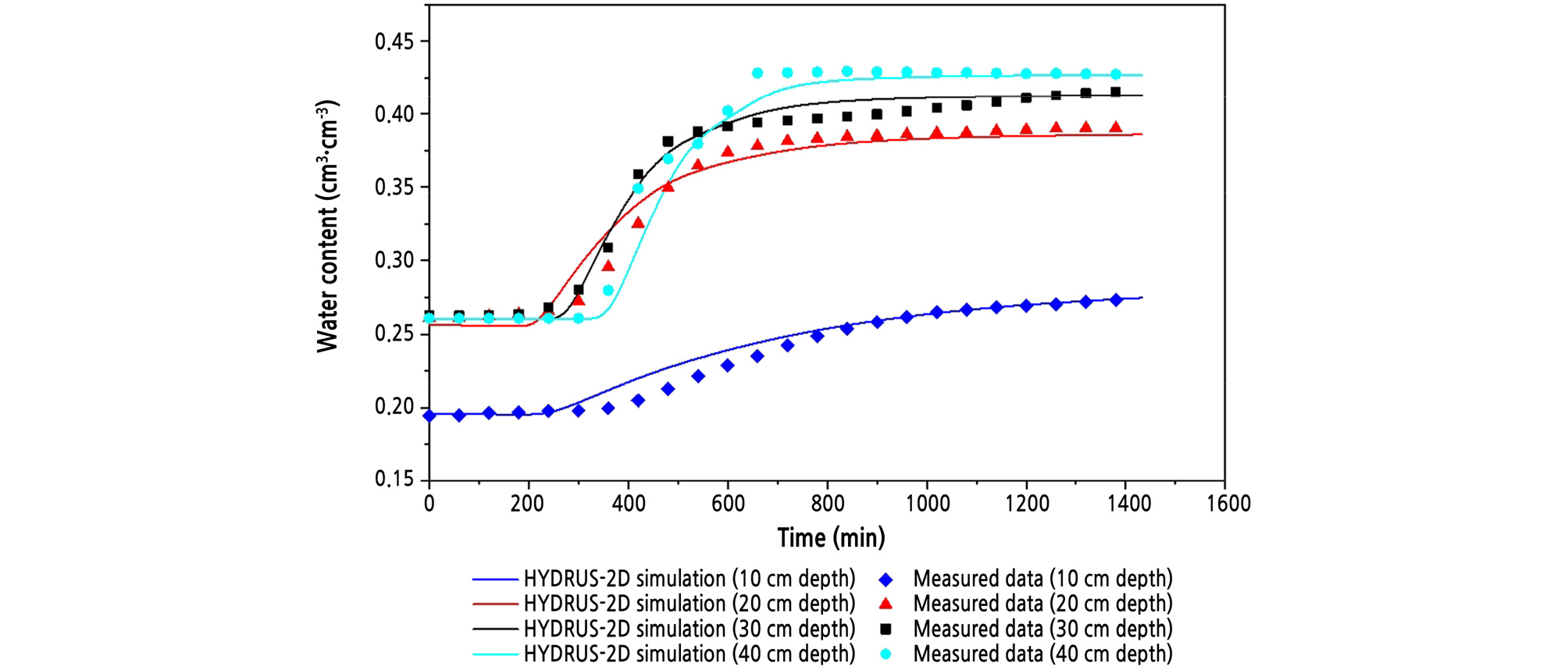
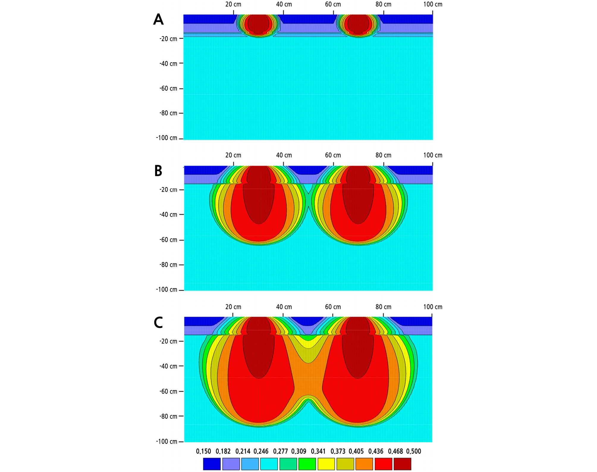
Fig. 3 shows the soil water contents at a 20-cm drip tube spacing and a comparison of these values with the HYDRUS-2D simulation. Because the distance between the emitter and the soil water sensor was relatively close (only 10 cm), the water content at a 10-cm depth began to increase 30 min after the start of irrigation and saturated at almost 200 min. As the sensing points became deeper, the reaching times increased linearly: 50 min at 20 cm, 80 min at 30 cm, and 110 min at 40 cm (Fig. 3). Fig. 4 shows the soil water distributions with irrigation time. The wetting patterns of the two adjacent emitters began to overlap at 150 min. As the irrigation time increased, they mutually interacted and moved downward predominantly.
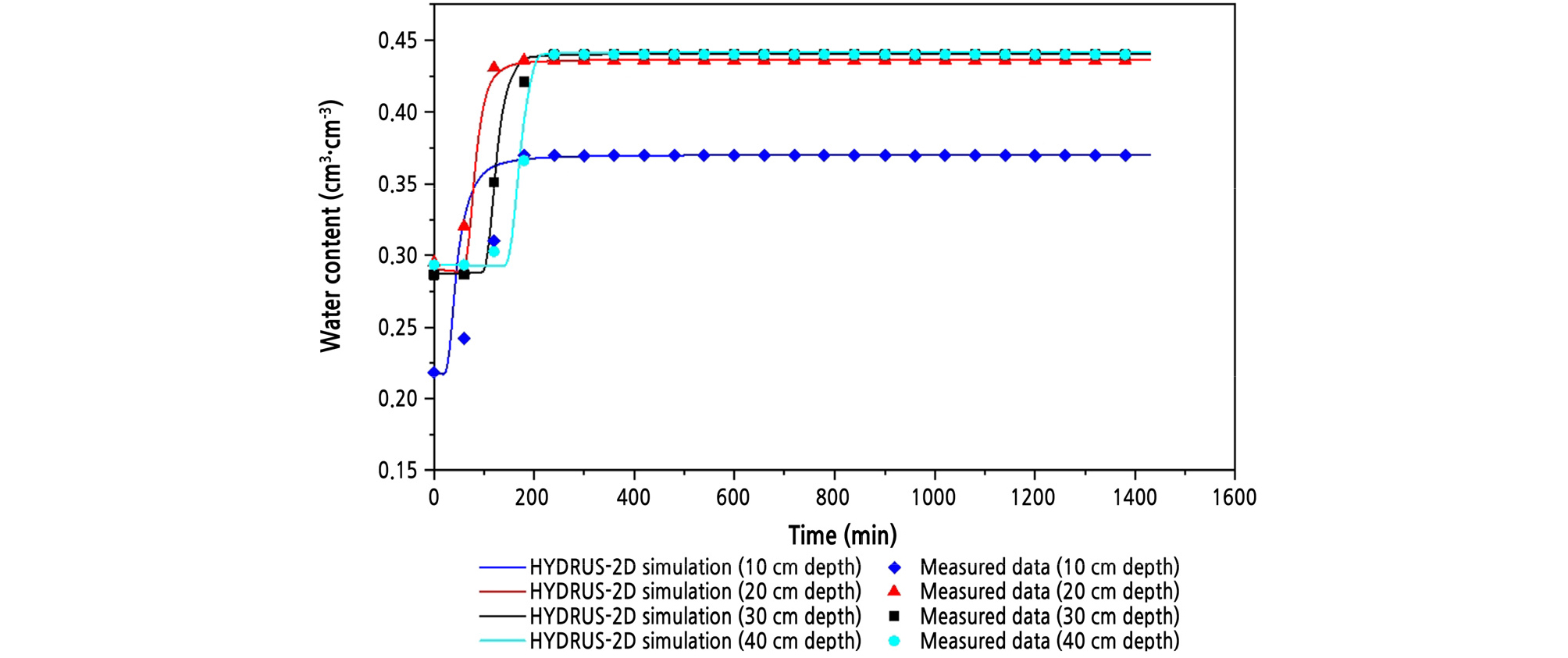
All the initial water contents, except at a 10-cm depth, were 29.0%, and the saturated water content was 43.9%, which is in the range of saturation water content of sandy loam soil (Soil Water Characteristics, Version 6.02.74, USDA ARS). However, at a 10-cm depth, the initial water content (21.8%) and the saturation water content (37.0%) were much lower than at other depths. This experiment was carried out using lysimeters 1 month after harvesting soybeans. Thus, because of the high organic matter content, the bulk density was low, so the saturation water content was significantly low. In addition, the sensor placed at a 10-cm depth showed lower values than the simulation (Fig. 3). This could have resulted from poor contact between the sensor and the soil from a lower bulk density. As a result, at this depth, RMSE, one of the error measures, was the largest among the depths. Conversely, R2 and E, the regression and efficiency measures, were the lowest (Table 3). However, the overall values (R2 = 0.948; RMSE = 0.011 cm3 cm-3; E = 0.946) showed satisfactory agreement between the measured and simulated data. In summary, irrigation with a drip tube spacing of 20 cm is effective for crops because it can provide water for the crop root zone for less than half an hour. However, in real cultivation, such a redistribution would be limited because of the crop’s soil water extraction.
Table 3.
Statistical comparison of measured and simulated data at dripline spacing of 20 ,40, and 60 cm
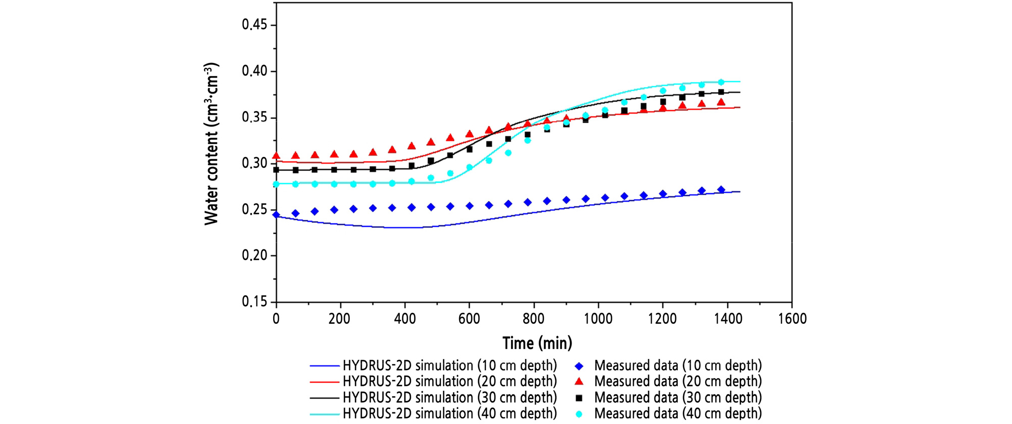
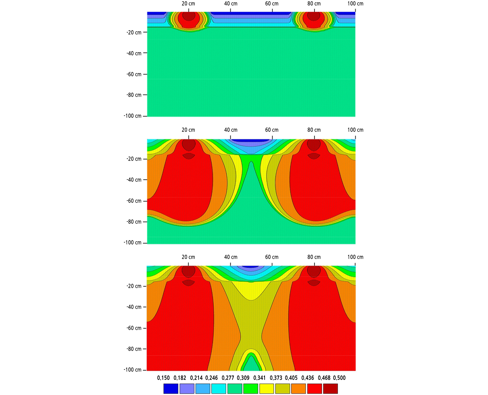
At a drip tube spacing of 40 cm, the emitter’s water took more time to reach the depths than the case with a drip tube spacing of 20 cm. In addition, the increasing rates () were much slower than at a drip tube spacing of 20 cm (Fig. 5). This is attributed to the higher elongation in the vertical direction compared with the horizontal direction (Fig. 6). Both wetting patterns were not met until 510 min, which is far slower than the time at the drip tube spacing of 20 cm (approximately 150 min). The wetting pattern continued to increase, and the wetting front reached the bottom at 960 min.
Similar to the drip tube spacing of 20 cm, the initial and saturation water contents at a depth of 10 cm were much lower than at the deeper ones. However, the saturation water contents at 20, 30, and 40 cm were not the same; this inconsistency may have been caused by inhomogeneity of soil characteristics along the vertical direction.
In addition, for all depths, the regression analysis (R2 = 0.989) and efficiency testing method (E = 0.988) indicated that the model accurately predicted the soil water content at a dripline spacing of 40 cm (Table 3). The error parameter (RMSE = 0.008) also remained within an acceptable limit.
At a drip tube spacing of 60 cm, the soil water content curves at all depths were somewhat different from those for the preceding spacing (Fig. 7). At depths of 20, 30, and 40 cm, the increasing rates of soil water content () were slowest, and the soil water contents continued to increase until the end of irrigation. This may be because of the elongation in the vertical direction and the relatively long distance (30 cm) between the emitter and the soil water sensor (Fig. 8). Both wetting patterns were observed at 900 min.
Similar to other drip tube spacings, at 10-cm depth, the soil water contents were low, and they showed almost constant values during the irrigation period. Water released from the emitter moved more vertically so that a small amount of water reached the region. In the simulation, the water contents decreased slightly by 500 min and then increased steadily. In the surface region, water tends to move downward because of gravity. The surface was also assumed in the model of a constant atmospheric boundary flux during time steps, which deviates from actual conditions at the surface boundary—that is, evaporation peaks in the daytime and decreases during the night (Ramos et al., 2012). R2 for the 10-cm depth was 0.837, which was lower than the other depths (Table 3). Conversely, E for a 10-cm depth was also −2.831, which indicates unacceptable performance (Moriasi et al., 2007). It can be concluded that the poorer correspondence between simulations and measurements at a 10-cm depth was most likely caused by the inadequacy of the soil hydraulic parameters. The performance parameters of other depths showed satisfactory agreement between measurements and simulations.
Drip tube spacing is one of the factors affecting vegetable growth. At a drip tube spacing of 20 cm, all soil depths were saturated with water within 200 min, which makes it possible to irrigate at the right time during the crop growing season. There was enough water in the root zone to be taken in by plant roots. However, at a drip tube spacing of 60 cm, irrigation water was less likely to contribute to the increase in water content midway between the emitters. However, plant development could not be particularly affected because the water content did not decrease. The effects of a dripline spacing of 40 cm were between those of 20- and 60-cm spacings.
For all drip tube spacings, R2 of 0.971, RMSE of 0.009 cm3 cm-3, and E of 0.959 were found between the measured and simulated water contents. Deviations between measured and simulated water contents can be attributed to field measurements and model input errors.
The source of error in field measurements is related to FDR measurements. FDR probes measure spatially averaged water contents over a certain soil volume, while simulation provides water content for a precise soil location (Ferre et al., 2002). Although the observation points (6 × 5 cm) were set at each depth to cover the area, this was not sufficient to represent highly nonuniform distribution areas, such as a depth of 10 cm. A wider area would give more representative values.
Another source of error in simulation is the uncertainty of soil hydraulic properties, which were taken from HYDRUS-2D. A nominal soil profile may not reflect the much larger simulated flow domain under experimental conditions. Moreover, the spatial and temporal variability of soil hydraulic properties was not considered in the simulation. Soil evaporation, which is an important factor in water flow simulation, also needs to be adjusted to experimental conditions. Considering these points in the simulation would improve the agreement between the measured and simulated data.
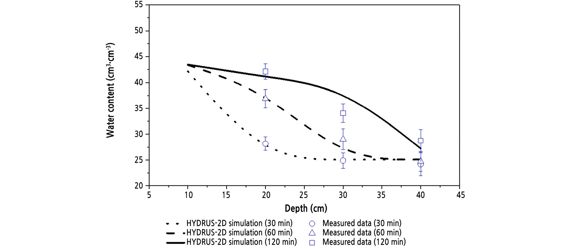
To verify the simulated soil water contents alternatively, we used the oven-drying method, which is a commonly used and convenient method to obtain a reasonable estimate of soil water content. When calibrating other types of water content measurements (e.g., FDR sensor), the oven-drying method is often regarded as having no error or uncertainty (Topp and Ferre, 2002). The soil water distributions under the emitters were simulated using HYDRUS-2D software. During the irrigation experiment, the soil samples were taken at 20-, 30-, and 40-cm depths, and their soil water contents were measured by the oven-drying method (105°C, 48 h). At 30 min, the simulation values were very close to the measured ones (Fig. 9). As time passed, the discrepancy increased slightly. However, the average relative error between the measured and simulated values was only 6.5%, which confirms the reliability of the simulated water content.
In farming, plastic mulching is used when growing crops. In this study, the experiment was performed when the amount of evaporation was low, so mulching was not considered, nor was it considered in the simulation process. However, since the amount of evaporation increases when crops are growing, plastic mulching greatly affects the behavior of soil water. When crops grow, without mulching, a water stress zone appeared in the 30- to 40-cm soil layer (Li et al., 2015).
In this study, soil water distribution was simulated without furrows or ridges. If we had used the exact geometry of ridges, we would have had more practical results for crop irrigation. However, soil water is mainly infiltrated in the direction of gravity and propagates in the horizontal direction; thus, similar water content distribution will be shown in the furrows or ridges. Therefore, by using the simulated soil water distribution, we can determine the optimal emitter distance for each crop. In addition, soil water distribution was simulated without crops. When crops grow, the amount of water that the roots absorb depends on the planting density and root area distribution. The simulation results show that, at crops with a planting distance of 20 cm, such as strawberries and lettuce (RDA, 2020), sufficient water could be supplied to the roots from a drip tube spacing of 20 cm. When the emitters are located between the crops and their distance is 40 cm, the water could be supplied to the crops efficiently, resulting in less water consumption.
Rockwool, a fibrous medium, and peat-based substrate mixtures have been widely used for plant cultivation as soilless substrates. Recently, the water movement characteristics of rockwool were investigated through an irrigation experiment (Choi and Shin, 2019) and the transpiration rate of paprika cultivated on rockwool was estimated by artificial neural networks (ANNs) (Nam et al., 2019). In addition, the flowers, petunia and zinnia, were grown in peat-based substrates with a high or low irrigation level, and their growth performances were analyzed by their irrigation levels (Choi et al., 2019). However, there aren’t studies available in scientific literature about the water distribution in soilless substrates. Therefore, the simulation model of water transport in soilless substrates along with the experiment, just like the approach in this study, would be helpful for developing an appropriate irrigation strategy.
Conclusions
Field experiments were performed to evaluate the water contents with different drip tube spacings when the wetting fronts were initially separated and later overlapped with time. The water contents were simulated continuously during the field experiment and compared well with measured experimental data, having an R2 of 0.97, RMSE of 0.009 cm3 cm-3, and E of 0.959. However, these values indicate much better performance than those from other simulation studies (Skagg et al., 2004; Kandelous and Šimůnek, 2010). This can be ascribed to the relatively simple simulation conditions, such as a short irrigation period, no root water uptake, and constant atmospheric boundary water flux. Under field conditions with surface drip irrigation, patterns of soil water content depend not only on drip tube spacing but also on the soil texture and emitter discharge rate. The latter, not examined in this study, could be evaluated by using model simulations, such as HYDRUS-2D.
Drip irrigation is an efficient method of applying water to horticultural crops. Irrigation scheduling is the process of determining how often to irrigate and how much water to apply. The main goal of irrigation is to provide the crops with the appropriate amount of water at the exact location, and precise soil water distribution can be obtained by simulation, which is difficult to perform using only field measurements. Once a simulation procedure is established using the field data, the modeling approach helps farmers adopt better irrigation management practices. In summary, this simulation approach using HYDRUS-2D was found to be a useful tool for simulating water infiltration in surface drip irrigation. However, three-dimensional simulation provides more realistic results.
